Collaborative filtering (CF) is one of the most popular techniques for building recommender systems. It is a method of making automatic predictions about the interests of a user by collecting preference or taste information from many users (collaborating). In this article, we will focus on memory-based algorithms and showcase some of our recent work on improving the classic CF implementation, thus making it applicable to large-scale datasets and reducing the training time by several magnitudes.

Memory-based algorithms can be divided into:

1. User-based CF: If we want to predict how user U will rate item I, we can check how other users who are similar to user U have rated that item. It is probable that the user will rate items similarly to users with similar tastes.
2. Item-based CF: If we want to predict how user U will rate item I, we can check how they have rated other items that are similar to item I. It is probable that the user will rate similar items similarly.

Let’s go through an example and see how user-based CF can be implemented. The following formulas show how to calculate rating ru,i, the prediction about how user u will rate item i. We aggregate over ratings that users similar to u have given to item i (the set of similar users is marked with S and the similarity function is marked with sim). The more similar a user is, the more influence his rating has on the overall prediction. The value of w is the weighting factor used to scale the sum down to a single rating.

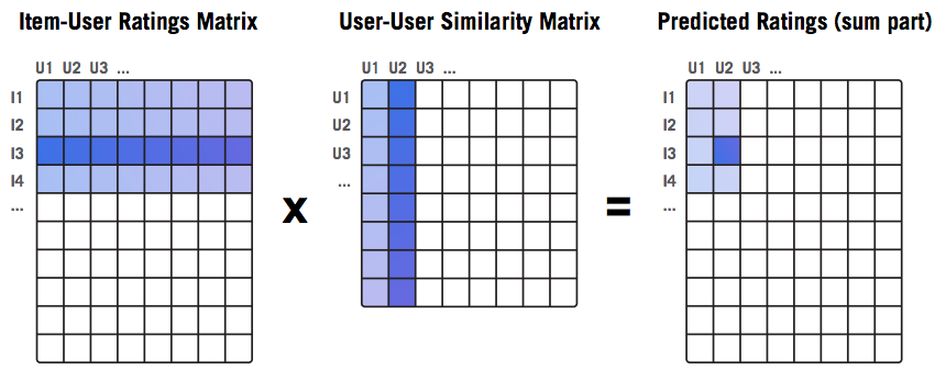
In order to evaluate a recommender system, we need to calculate the predictions for all ratings in a test set. Calculations are usually not done in a loop, but rather using matrix multiplication since it is a much faster operation. The following picture shows the matrices being used:

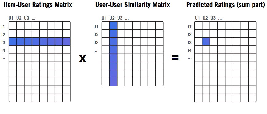
Let’s focus on user U2 and item I3 for a moment. For predicting how user U2 will rate item I3, we need to know how other users have rated I3 (the blue row in the first matrix) and how similar other users are to U2 (the blue column in the second matrix; note that the similarity of U2 to itself can be ignored by setting it to zero). In this case, the formula for the sum from above can be written as follows (user and item are marked as u2 and i3, and set S covers all users):

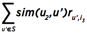
The result is stored in the blue cell of the rightmost matrix.In order to find the final prediction, we also need the coefficient w (as explained above), which is calculated in a similar manner. Finally, by multiplying two matrices, we get instant results for all predictions (not only for U2, I3).

One of the main disadvantages of memory-based CF is related to its scalability and performance when matrices are large. We tried to address these issues using a new implementation of CF in the R programming language (this can be applied to other languages as well). Our implementation was compared to one of the most commonly used packages for recommender systems in R, ‘recommenderlab’. The comparison was performed on a single computer with a 4-core i5 and 16GB of RAM using well-known and freely available datasets (MovieLens 1m and MovieLens 10m). It will be shown that our implementation:

• Is significantly faster.
• Can support building recommender systems on large datasets, for which the ‘recommenderlab’ implementation runs out of memory.

Execution Time Improvement

Ratings matrices are usually both large (there are a lot of users and items) and sparse (users typically rate only a few items, if any). In R, there is a special representation for sparse matrices, such that missing values (ratings) are not stored into memory. Very often, over 90% of ratings are missing, so this saves a lot of memory. Our implementation, as well as ‘recommenderlab’, uses this sparse form of matrices.

The main steps used in our implementation of user-based CF are as follows (the same approach is used for item-based CF):

Take a ratings matrix.

1. A user specifies whether to normalize ratings. This step usually increases accuracy. Normalization is used to remove individual ratings bias, which is introduced by users who consistently give lower or higher ratings compared to other users.
2. Calculate similarities between users.
3. Use the k nearest neighbor approach (keep only k most similar users by keeping only k highest values per columns in the user-user similarity matrix). The user needs to specify the value of k.
4. Calculate predictions and denormalize them in case normalization is performed in step one.

The implementation in ‘recommenderlab’ follows the same procedure. However, we have introduced optimizations that have resulted in significant speed improvements. The two main optimization steps are summarized below:

1. Similarities are calculated using R functions that operate on sparse matrices.
2. k-nearest neighbors on similarity matrices were not calculated in a loop, but rather using an optimized implementation. First, we grouped all the values from the similarity matrix by column. In each group (column), we applied a function that finds the k-th highest value. This was implemented using the R ‘data.table’ package. Finally, we used this information to keep only the k highest values per column in the similarity matrix.

Evaluation

We compared our implementation vs. ‘recommenderlab’ using the following setup:

• 10-fold cross validation. In each iteration, 90% of the ratings were used to create the model and calculate similarities and 10% were used for testing. All users and items were considered for both training and testing.
• Center normalization, where user’s average rating is subtracted from his actual ratings.
• Cosine measure to calculate similarities.
• k: the number of nearest neighbors was set to 100 and 300.

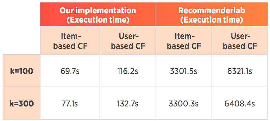
The evaluation was performed on a popular MovieLens 1m dataset. This dataset contains 6,040 users and 3,706 movies (items), with 1,000,209 ratings. The results can be found in the table above, showing execution time of the algorithm in seconds.

As it can be seen, we have achieved a significant speedup. However, the speed is only one side of the problem with this classic implementation. As we have already mentioned, another concern is space, i.e. what to do whenwe run out of memory in case matrices become too large. In the next section, we will introduce a new approach to make it feasible to train CF recommender even on large datasets, on which classic implementation might run out of memory.

Build a Recommender on Large Datasets

In this test, we used the MovieLens 10m dataset. Just to recall, all algorithms were run on a single machine with16 GB of RAM and evaluated using 10-fold cross validation.In such a setup, the ‘recommenderlab’ implementation cannot be used on this data set (at least for user-based CF, since it runs out of memory when the similarities matrix needs to be calculated).

In our implementation, we tried to solve the problem of large matrices by dividing them into parts, i.e. we did not calculate all predictions at once but in chunks. Here is the procedure for user-based CF (the same approach is used for item-based CF):

1. Take N rows (items) of the item-user matrix. In the picture, we took rows of indices [I1:I4].
2. Take M users and calculate similarities between them and all other users. In the picture, we calculated similarities for users [U1:U2].
3. Calculate the product of N rows from step 1 and M columns from step 2. The result is the MXN matrix, which contains the sums used to find the predictions.In our example, those will be predictions about how items I1 to I4 will be rated by users U1 and U2.
4. Repeat the first three steps for different N and M chunks until the result matrix is fully covered.

Results on MovieLens 10M Dataset

This dataset contains 69,878 users and 10,677 movies with around 10,000,054 ratings. Here is the evaluation setup:

• 10-fold cross validation, as explained above.
• Center normalization.
• Cosine measure to calculate similarities.
• k: The number of nearest neighbors was set to 100and 1000.
• Chunk size: The numbers of rows and columns per chunk are the parameters of the algorithm. We used some values that we found to be nearly optimal for our hardware setup.

The results of the comparison can be found in the following table, showing the execution time of the algorithm in minutes.

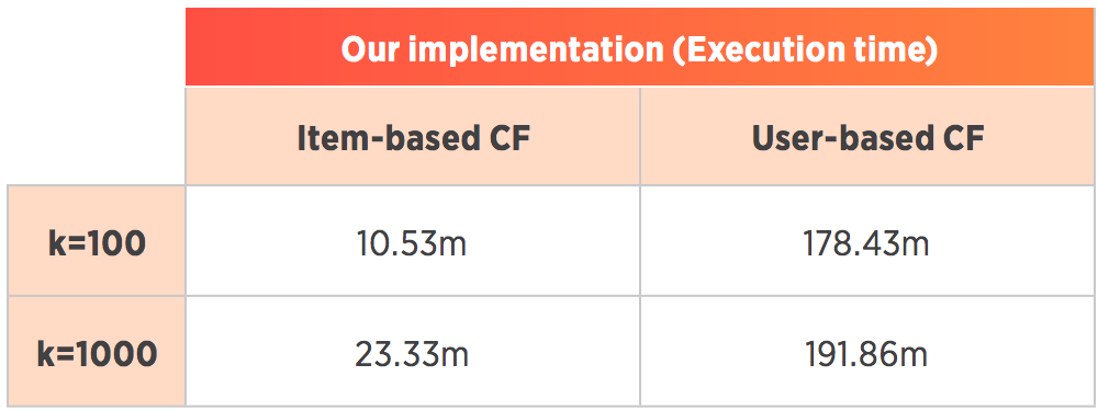
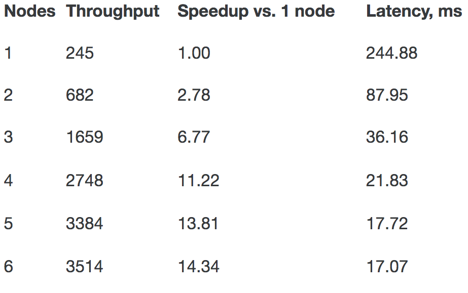
As we can observe, the algorithm was executed successfully. With this current implementation, when we need to find recommendations in real-time for one or several users, the calculation of similarities and predictions will be much faster, since we will operate on a small number of users. On the MovieLens 10m dataset, user-based CF takes a second to find predictions for one or several users, while item-based CF takes around 30seconds. This can be optimized further by storing the similarity matrix as a model, rather than calculating it on the fly. Additionally, an obvious advantage of this algorithm is that it is scalable. Since we calculate predictions on chunks of matrices independently, it is suitable to be parallelized. One of the next steps is to implement and test this approach on some distributed framework. The code is freely available as a public GitHub project. In the near future, we plan to work on this implementation further, extend the project with new algorithms, and possibly publish it as an R package.